A Reversi Playing Agent and the Monte Carlo Tree Search Algorithm
Play against a Reversi (Othello) AI implemented with the Monte Carlo Tree Search (MCTS) Alogrithm.
- Monte Carlo Tree Search
- Go, Javascript
The Monte Carlo Tree Search (MCTS) algorithm has garnered much attention over recent years for its application in creating auntonomous agents that can achieve high-level play for perfect information, deterministic games. Here, you get to play against the MCTS Reversi (Othello) agent that I built. This post will also discuss the assessment of this algorithm's level of skill, followed by a walkthrough of my implementation of the MCTS agent, and the variations applied to the algorithm in this context. But first, you may want to pit your skills against the agent below. You can check out the source code at https://gitlab.com/royhung_/reversi-monte-carlo-tree-search.
Reversi MCTS Agent
nSims=50, Iterations=200
Pedants may point out that Reversi and Othello are different games. However, the differences are mostly inconsequential, such as the starting positions of the pieces. For our purposes, the rules of the game in our context follow the official "Othello" rules, and we will use the term "Reversi" and "Othello" interchangeably going forward.
Summary of Results
How well does the algorithm play? In Fig. 1, the performance of this algorithm is benchmarked against a pseudo-random algorithm. A variation of the MCTS algorithm that incorporates domain knowledge (i.e, hard-coded with heurstic rules) was also tested and the results compared.
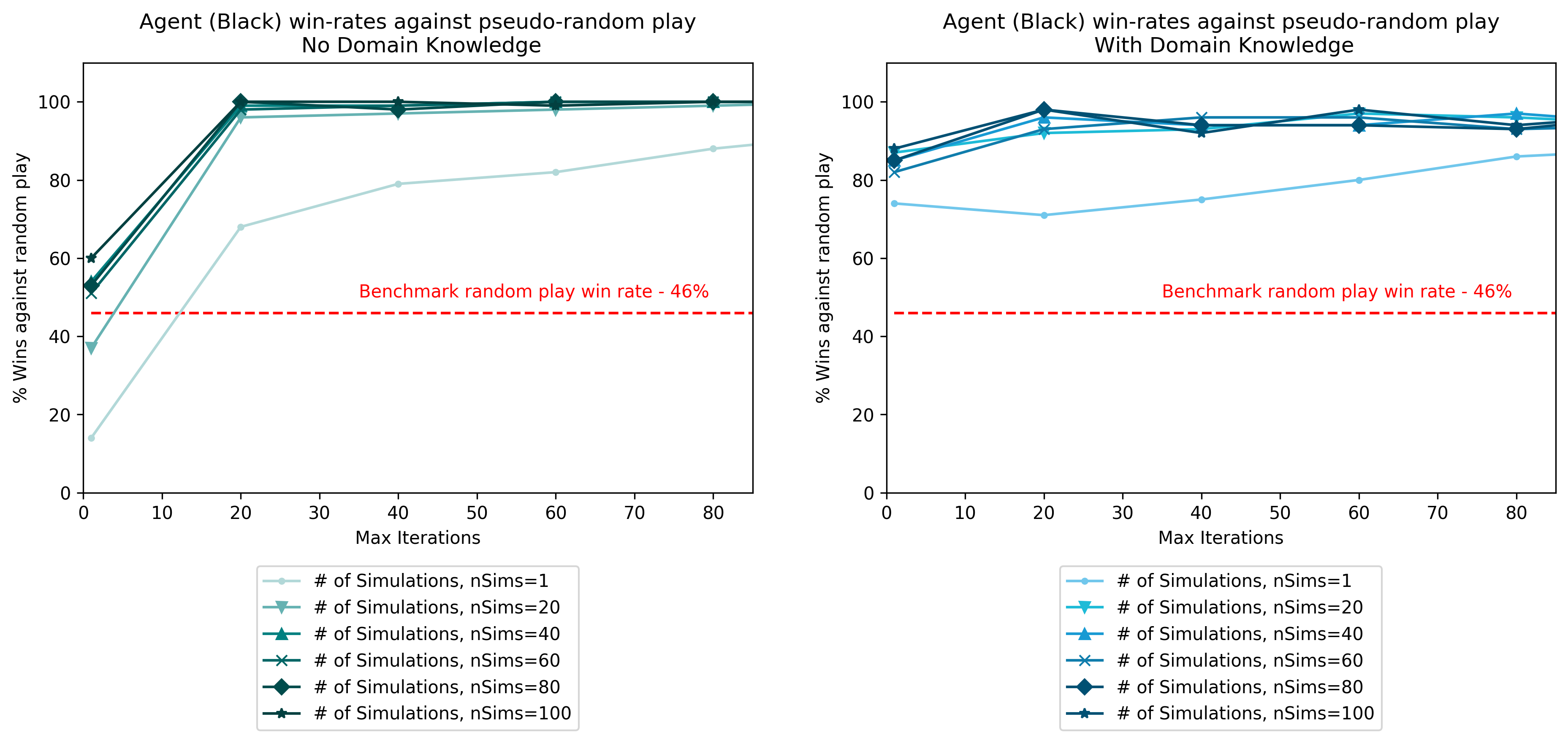
Fig. 1 - Agent win rates against pseudo-random play
In Fig. 1, the MCTS agent plays black and has a benchmark win rate of 46% to beat. This benchmark is the empirical win rate for black if both sides play randomly. It turns out that the algorithm, even with a low number of iterations (max_iter) and a low number of games simulated (nSims) per node, can easily beat a random-play algorithm. At 40 iterations onwards, it achieves a consistent win rate of >99%.
A more interesting finding is the performance of MCTS when supplemented with domain knowledge. The incorporation of domain knowledge nudges the algorithm to favor making moves that are generally considered good moves, according to human experience. The results show that incorporating domain knowledge dramatically improves win rates when the the MCTS algorithm has less iterations, and less games simulated. However, at higher iterations, domain knowledge has in fact, led to lower win-rates (~97%). This seems to suggest that the rigid heuristics that come with domain knowledge can serve to impede rather than aid the algorithm especially in late-game play, where simulations from an unassisted MCTS can easily determine the winning solution.
Despite how easily the algorithm can beat pseudo-random play, it does not fare very well against human players in general (Did you manage to beat it?). Augmented with domain knowledge, the MCTS agent can pose a formidable challenge to novice players in early-mid game. Nevertheless, even if it does not make any discernibly bad moves, it fails to capitalize on winning opportunities, and is unable to implement basic strategies, such as forming wedges, or creeping along edges. These missed opportunities, together with its propensity to make some weak moves in mid-game, ultimately make it a fairly easy opponent to beat.
Monte Carlo Tree Search
There are plenty of excellent resources on the Internet explaining the MCTS algorithm in great depth. As such, I wlll not cover the basics in detail here. Instead, I will give a high-level overview behind the intuition of each stage of the algorithm, and focus on the variations that I have applied for this reversi agent.
In a nutshell, the MCTS algorithm iteratively searches a tree structure where each node in the tree represents the outcome, or game state following from the previous game state (i.e., the parent node). The tree is grown by adding nodes each time the algorithm traverses down the tree and reaches a leaf node. This process of adding nodes is called the expansion phase.
Each iteration of the MCTS algorithm goes through the following 4 phases, and the algorithm stops iterating after the number iterations exceeds a user-determined parameter, which we will refer to as max_iter here. The procedure for one iteration is as follows:
- Selection
- Expansion
- Simulation
- Backpropagation
1. Selection
The selection phase determines how the algorithm should choose the child node to traverse down the tree. In other words, when searching for the best move to make, which node is the most promising to look into? Here, the Upper Confidence Bound applied to trees (UCT) algorithm is used. Each node contains a UCT score and the algorithm will select the node with the highest UCT score.
UCT= \frac{w_i}{n_i} + c\sqrt{\frac{\ln N}{n_i}}
w_i : The number of wins simulated in node i
n_i : The number of simulated games in node i
N : The total number of simulated games
c : Exploration constant
Tweak the exploration constant to set how "adventurous" the algorithm can be. A high value will nudge the algorithm to select a node that has been rarely visited. The UCT calculation can be further supplemented by domain knowledge, to further encourage the algorithm to make better moves, according to human experience, or to at least avoid making disastrous moves that give the game away.
2. Expansion
After selecting a child node, the algorithm enters the expansion phase where it adds new, unexplored child nodes to the selected child node. These nodes represent all the valid moves (game states) that can be made on that child node.
3. Simulation
In the selected child node, the simulation phase takes place. The objective of this phase is to playout the rest of the game to completion, from the current game state. For this reversi agent, a pseudo-random play algorithm is used for both sides and the number of wins w_i out of the number of simulations n_i is tabulated and recorded in the node itself. It is worthwhile to point out that at there are other ways to implement this stage. In some applications, the simulation phase uses the MCTS algoritm itself as its own simulated opponent and the entire tree is replicated for one simulation. The obvious tradeoff in doing so is the high computational cost, as compared to using a random play algorithm on both sides which can be simulated quickly, allowing for higher number of simulations.
Yet, the downsides of using random play for the rollout of the simulation stage is also apparent. While computationally cheap, the moves made are all random on both sides. For a game like Reversi, randomly giving away a corner piece is generally considered a bad move in most cases, and this agent's decision-making ability will be built upon such terrible strategies. As such, for this reversi agent, a slight compromise was made and a pseudo-random playout is used to discourage making disastrous moves for both sides during simulations.
func simRand(game Board) Board {
    // Given a Board, simulate all moves randomly until end of game
    for {
        if game.winner == 0 {

            //rand is deterministic. Need to set seed
            rand.Seed(time.Now().UTC().UnixNano())
            move := game.validSpace[rand.Intn(len(game.validSpace))]
            game.Move(move)
        } else {break}
    }
    return game
}

func simRandPlus(game Board) Board {
    // Given a Board, simulate all moves semi-randomly until end of game
    // Added heuristic to discourage making very bad positions during rollouts
    // Both sides in simulation will avoid very bad positions
    // Alternative to default simRand function
    for {
        if game.winner == 0 {

            //rand is deterministic. Need to set seed
            rand.Seed(time.Now().UTC().UnixNano())
            move := game.validSpace[rand.Intn(len(game.validSpace))]

            // When a very bad position is chosen,
            // Choose again, repeat again if very bad position chosen
            if posInSlice(move, veryBadPositions) == true {
                move = game.validSpace[rand.Intn(len(game.validSpace))]
                if posInSlice(move, veryBadPositions) == true {
                    move = game.validSpace[rand.Intn(len(game.validSpace))]
                }
            }
            game.Move(move)
        } else {break}
    }
    return game
}
In the code block above, the function simRandPlus was used for the algorithm as opposed to simRand. If a pre-determined "bad position" was selected randomly, the random selection is repeated. This reduces the chance of a bad move being made unless it is the only valid move available. It is also a computationally cheap variation to make.
| Table 1: Comparison of the number of games won by colour and algorithm | |||
| White | |||
| Black | Random | Pseudo-Random | |
| Random |
B: 4,604 W: 4,985 D: 411 |
B: 3,698 W: 5,933 D: 369 |
|
| Pseudo Random |
B: 5,479 W: 4,128 D: 393 |
B: 4,655 W: 4,985 D: 360 |
|
| Total Played | 10,000 | 10,000 | |
| Note: B, W, D, stand for number of games won by Black, number of games won by White, and number of Draws respectively. The side with more wins is highlighted in yellow. |
|||
To test the effectiveness of going pseudo-random, we pit the two playout algorithms against each other in Table 1. Interestingly, in a pure random play, the second player (white) seems to have a slight advantage over the first player (black). This seems to suggest a second mover advantage. With both players using the pseudo-random algorithm, white edges out more wins again.
It is also clear that the pseudo-random algorithm is a stronger one. For the matchups of pseudo-random algorithm versus pure random, pseudo-random racks up over a thousand more wins, regardless of the starting colour. A simple heuristic applied to the random play algorithm simply to reduce the probability of picking a disastrous position has yielded quite significant improvements in win-rates.
It is possible to further supplement this pseudo-random algorithm with even more domain knowledge. Here, we only tweak the algorithm to avoid giving away corners. There are other, less terrible positions to avoid which we can also incorporate into the algorithm. How about favoring generally good positions? Or edge pieces? There are many more ways to experiment with these heuristics for the playout algorithm.
4. Backpropagation
In the final stage of MCTS, the algorithm traverses back up the tree and increments each node the number of wins, losses, and games played until the parent node is reached. This completes one iteration of the MCTS algorithm.
It is also worth pointing out that information other than the number of wins and losses can also be backpropagated up the tree. One piece of information that could also be backpropagated is the concept of "mobility" in Othello. There are many measures of mobility, but in essence, they represent the sum total of legal moves you can make. The more legal moves available to the player (i.e., higher mobility), the better. Conversely, in a situation of low mobility, the player has little moves to make, and may be forced by the opponent to make a bad move, such as giving up a corner. As such it is generally a good strategy to optimize for mobility.
Simply counting the number of legal moves in the current game state would be a poor indication of the mobility in future game states. That is why if we can calculate the mobility for each game state down the tree, backpropagate and aggregate them at the parent node, the statistic could be used to supplement the decision making for the agent.
func backProp(n *Node, wins int, loss int, played int ) {

    // Backpropagation to traverse from child to parent nodes
    // Update count of wins and played games starting from Node n
    turn := n.state.turn
    mobility := float64(len(n.state.validSpace))
    for {
        if n.state.turn == turn {
            n.wins += wins
            n.mobility += mobility
        } else {
            n.wins += loss
        }
        n.played += played
        if n.parent == nil {
            break
        } else {
            n = n.parent
        }
    }
}
Selecting the Best Move + Domain Knowledge
After MCTS completes its iterations. It is time for the agent to make an informed decision on which of the legal moves to pick. In a vanilla implementation of the algorithm, the UCT score for the immediate child nodes are compared and the node with the highest UCT score is selected as the agent's next move. Intuitively, this makes sense as the UCT method favors the node that has produced the most wins (barring the exploration term). However, if the search depth is not deep enough, or the number of simulations too low. UCT may fail to select good moves. And this was also reflected in the results in Fig. 1 where MCTS with insufficient simulations/search depth can perform worse than random play (nSims=1, max_iter=1).
UCT also tends to perform poorly in early-mid games as the search space is too large. As such, incorporating heuristic rules, or domain knowledge to aid the algorithm has the potential to make it a much better player. These heuristics are calculated statistics (other than wins/losses) that alter the final UCT score by penalizing or augmenting the raw UCT scores. The equations below show the adjustments that this reversi agent uses.
Preference for Inner Pieces
InnerScore_{i,j} = \frac{a \cdot UCT_{i,j}}{\sqrt{(i-3.5)^2 + (j-3.5^2)}}
Where 0 \leq i, j < 8
This is a positive reinforcement to nudge the agent into favoring moves that are closer to the center. i, j refer to a given position (ith row and jth column) of the move on the board. When i or j is high, it means that the position is nearer to the edge, resulting in a lower InnerScore . a is the weight to be given to InnerScore.
Greed Penalty
GreedPenalty_{i,j} = \frac{(-1)^t \cdot (blackScore_{i,j} - whiteScore_{i,j})}{(blackScore_{i,j} + whiteScore_{i,j})^b}
Where 0 \leq i, j < 8
t = \begin{cases} 1 &\text{if Agent plays black} \\ -1 &\text{if Agent plays white} \end{cases}
It is generally not a a good idea to be flip too many pieces in early-mid game, as this would result in lower mobility, giving your opponent a larger pool of legal moves to make. As such, we can penalize being greedy in the early part of the game, and reduce this penalty towards the later part of the game (hence the denominator). b is a tweakable parameter to determine the weight of the penalty towards the end game.
Position Penalty
PositionPenalty_{i,j} = \begin{cases} c \cdot UCT_{i,j} &\text{if } i=1, j=1 \\ c \cdot UCT_{i,j} &\text{if } i=1, j=6 \\ c \cdot UCT_{i,j} &\text{if } i=6, j=1 \\ c \cdot UCT_{i,j} &\text{if } i=6, j=6 \\ d \cdot UCT_{i,j} &\text{if } i=0, j=1 \\ d \cdot UCT_{i,j} &\text{if } i=1, j=0 \\ d \cdot UCT_{i,j} &\text{if } i=6, j=0 \\ d \cdot UCT_{i,j} &\text{if } i=7, j=1 \\ d \cdot UCT_{i,j} &\text{if } i=7, j=6 \\ d \cdot UCT_{i,j} &\text{if } i=6, j=7 \\ d \cdot UCT_{i,j} &\text{if } i=0, j=6 \\ d \cdot UCT_{i,j} &\text{if } i=1, j=7 \\ \end{cases}
Where 0 \leq i, j < 8
0 \leq d \leq c < 1
The penalty for making these pre-determined "bad" moves is a simple percentage of the raw UCT score. c and d determine the penalty weights for x-square positions (adjacent to the corners diagonally) and c-square positions (adjacent to the corners on the edges) respectively.
Final Adjusted UCT Score
UCTFinal_{i,j} = UCT_{i,j} + InnerScore_{i,j} - GreedPenalty_{i,j} - PositionPenalty_{i,j}
The final UCT score that the agent will used to decide the next move is given as the raw UCT score plus any augmentations and less any penalties. The child node with the highest UCTFinal_{i,j} score is selected as the move to make.
Performance Issues
In terms of improving computation speed of this reversi agent, much more could be done. The current version of this agent employs the MCTS algorithm even for the opening moves. This is a futile effort considering the search space is too large for the algorithm to come up with a decent opening strategy. What most Othello applications do here is to use a predefined opening playbook, thus speeding up the decision making for the early part of the game.
In addition, the tree structure built by the MCTS algorithm does not persist between game states. That means the algorithm will rebuild the entire tree for every move. We can do better by allowing the current state of the tree to be saved and loaded between moves according to each unique game session. Doing so will also improve the quality of the UCT score as the backpropagated statistics for each node can be accumulated across game states.
Conclusion
The MCTS algorithm, by itself is not enough to be a formidable opponent to a human player. To improve its ability, simply turning up the number of iterations and simulations for this agent may work, albeit at the cost of computation time. But the marginal returns to increasing iterations and simulations will diminish quickly, and the skill ceiling of a vanilla MCTS algorithm will be made apparent. To futher strengthen it, domain knowledge can be applied, and this opens up an many more possibilities. As each additional heuristic that augments the algorithm come with more dials and knobs to optimise.
Despite its shortcomings, MCTS remains a novel and effective alternative to more traditional, deterministic algorithms that tend to evaluate every possible move. Put in this comparison, MCTS is in fact a smarter way to navigate an unbounded search space.